Choice Platform Options

Choice Model red triangle menu contains the following options.

Note: When you use Hierarchical Bayes, the subject-level estimates are based on Monte Carlo sampling. For this reason, results obtained for the options below vary from run to run.

Likelihood Ratio Tests

See Likelihood Ratio Tests.

(Available for Hierarchical Bayes) Shows non-Firth maximum likelihood estimates and standard errors for the coefficients of model terms. These estimates are used as starting values for the Hierarchical Bayes algorithm.

Joint Factor Tests

(Not available for Hierarchical Bayes) Tests each factor in the model by constructing a likelihood ratio test for all the effects involving that factor. For more information about Joint Factor Tests, see Joint Factor Tests in Fitting Linear Models.

Confidence Intervals

(Not available for Hierarchical Bayes) Shows or hides a confidence interval for each parameter in the Parameter Estimates report.

Confidence Limits

(Available for Hierarchical Bayes) Shows or hides confidence limits for each parameter in the Bayesian Parameter Estimates report. The limits are constructed based on the 2.5 and 97.5 quantiles of the posterior distribution.

Correlation of Estimates

If Hierarchical Bayes was not selected, shows the correlations between the maximum likelihood parameter estimates.

For Hierarchical Bayes, shows the correlation matrix for the posterior means of the parameter estimates. The correlations are calculated from the iterations after burn-in. The posterior means from each iteration after burn-in are treated as if they are columns in a data table. The Correlation of Estimates table is obtained by calculating the correlation matrix for these columns.

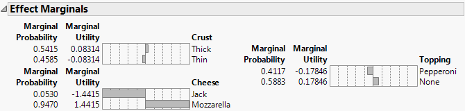
Effect Marginals

Shows or hides marginal probabilities and marginal utilities for each main effect in the model. The marginal probability is the probability that an individual selects attribute A over B with all other attributes set to their mean or default levels.

In Figure 4.18, the marginal probability of any subject choosing a pizza with mozzarella cheese, thick crust and pepperoni, over that same pizza with Monterey Jack cheese instead of mozzarella, is 0.9470.

Figure 4.18 Example of Marginal Effects 

Utility Profiler

Shows or hides the predicted utility for different factor settings. The utility is the value predicted by the linear model. See Find Optimal Profiles for an example of the Utility Profiler. For more information about utility, see Utility and Probabilities. For more information about the Utility Profiler options, see Prediction Profiler Options in Profilers.

Probability Profiler

Enables you to compare choice probabilities among a number of potential products. This predicted probability is defined as follows:

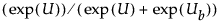
where U is the utility for the current settings and Ub is the utility for the baseline settings. This implies that the probability for the baseline settings is 0.5. See Utility and Probabilities.

See Comparisons to Baseline for an example of using the Probability Profiler. For more information about the Probability Profiler options, see Prediction Profiler Options in Profilers.

Multiple Choice Profiler

Provides the number of probability profilers that you specify. This enables you to set each profiler to the settings of a given profile so that you can compare the probabilities of choosing each profile relative to the others. See Multiple Choice Comparisons for an example of using the Multiple Choice Profiler. For more information about the Multiple Choice Profiler options, see Prediction Profiler Options in Profilers.

Comparisons

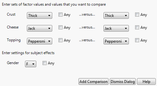
Performs comparisons between specific alternative choice profiles. Enables you to select the factors and the values that you want to compare. You can compare specific configurations, including comparing all settings on the left or right by selecting the Any check boxes. If you have subject effects, you can select the levels of the subject effects to compare. Using Any does not compare all combinations across features, but rather all combinations of comparisons, one feature at a time, using the left settings as the settings for the other factors.

Figure 4.19 Utility Comparisons Window 

Willingness to Pay

Requires that your model includes a continuous price column. Calculates the maximum price increase (decrease) that a customer is willing to pay for a new feature over the baseline feature cost. The result is calculated using the Baseline settings for each background setting.

Save Utility Formula

When the analysis is on multiple data tables, creates a new data table that contains a formula column for utility. The new data table contains a row for each subject and profile combination, and columns for the profiles and the subject effects. When the analysis is on one data table, a new Utility Formula column is added.

Save Gradients by Subject

(Not available for Hierarchical Bayes.) Constructs a new table that has a row for each subject containing the average (Hessian-scaled-gradient) steps for the likelihood function on each parameter. This corresponds to using a Lagrangian multiplier test for separating that subject from the remaining subjects. These values can later be clustered, using the built-in-script, to indicate unique market segments represented in the data. See Gradients. For an example, see Example of Segmentation.

(Available for Hierarchical Bayes.) Creates a table where each row contains the subject-specific parameter estimates for each effect. The distribution of subject-specific parameter effects for each effect is centered at the estimate for the term given in the Bayesian Parameter Estimates report. The Subject Acceptance Rate gives the rate of acceptance for draws of new parameter estimates during the Metropolis-Hastings step. Generally, an acceptance rate of 0.20 is considered to be good. See Bayesian Parameter Estimates.

(Available for Hierarchical Bayes.) Creates a table that gives information about the chain of iterations used in computing subject-specific Bayesian estimates. See Save Bayes Chain.

Model Dialog

Shows the Choice launch window, which can be used to modify and re-fit the model. You can specify new data sets, new IDs, and new model effects.

See Redo Menus and Save Script Menus in Using JMP for more information about the following options:

Redo

Contains options that enable you to repeat or relaunch the analysis. In platforms that support the feature, the Automatic Recalc option immediately reflects the changes that you make to the data table in the corresponding report window.

Save Script

Contains options that enable you to save a script that reproduces the report to several destinations.

Save By-Group Script

Contains options that enable you to save a script that reproduces the platform report for all levels of a By variable to several destinations. Available only when a By variable is specified in the launch window.