Findings Shift Plots
The Findings Shift Plots Report supports exploratory review of changes in continuous findings measurements between baseline and the on-treatment period. It can be used with data from a variety of domains, including Laboratory Test Results(LB), Vital Signs (VS), ECG Results (EG) and findings data represented in analysis domains such as ADEF and ADMRI.
The report compares each subject’s baseline value with a summarized post-baseline value through a matched pairs analysis. Flexible options are available for defining both baseline and post-baseline measurements. Baseline may be defined using the last pre dose assessment, the mean of pre-dose assessments, or a value identified by a baseline flag. Post-baseline values may be summarized using the mean, minimum, maximum, median, or last available on-treatment measurement.
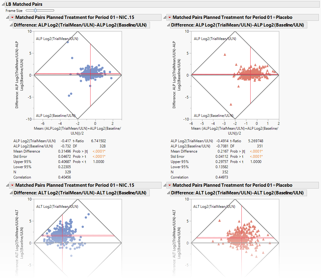
The report can be used to evaluate shifts from baseline within and between treatment groups, assess the magnitude and direction of change, and identify subjects with notable or outlying responses that may warrant further review. Visual patterns in the shift plots can help reviewers detect trends, potential safety signals, treatment-related effects, and subpopulations with atypical responses.
Note: JMP Clinical uses a special protocol for data including non-unique Findings test names. Refer to How does JMP Clinical handle non-unique Findings test names? for more information.
Methodology
No testing is performed. Analysis is restricted to calculating simple statistics of post-baseline findings results or their log transformed and/or normalized values against baseline values.
Usage and Interpretation
The Findings Shift Plots Report is intended for exploratory data review. Observed patterns may generate hypotheses or identify areas for additional investigation, but the visualizations are not intended to provide formal statistical inference. Reviewers can drill down from plotted observations to subject-level details, enabling rapid investigation of potentially clinically meaningful changes.
The following examples illustrate common clinical review scenarios and demonstrate how shift plots can support efficient identification and evaluation of potential findings of interest.
Note: Click on the figures below to enlarge.
Example 1: Baseline vs Mean Blood Urea Nitrogen (BUN) Concentration by Treatment
In this example, report options were set as shown in the following table:
| Option Type | Option | Setting | |
|---|---|---|---|
| Display | Laboratory Test Results | Blood Urea Nitrogen (mMol/L) | 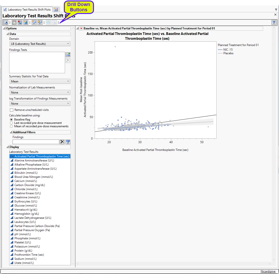
|
|
All other options are set to default. |
|||
This example coincides with Example 1 in the Findings Time Trends report documentation, and Example 1 in the Findings Box Plots report documentation graphs the baseline verses the Mean Post-baseline Blood Urea Nitrogen (BUN).
Figure 1: Baseline vs. Mean Post-baseline BUN
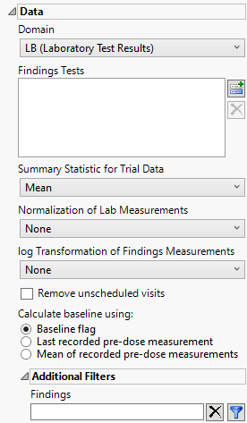
Figure 1 compares baseline BUN values with mean post-baseline BUN values for each subject. Many observations occur above the line of equality, suggesting that BUN values tended to increase during treatment. The wide spread of post-baseline values indicates substantial variability across subjects. A small number of observations are separated from the main cluster, indicating subjects whose BUN values may warrant additional review.
The distribution of post-baseline BUN values is right-skewed, causing many observations to appear compressed within a small area of the plot. Applying a log transformation can improve visualization by spreading observations more evenly across the plotting space, making treatment-group patterns and potential outliers easier to identify. To apply the log transformation, from the Data option, we select “Log 2 (for the log (base 2) transformation) using the Log Transformation of Findings Measurements drop down menu.
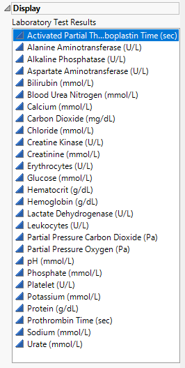
Figure 2 displays the same data after applying the log2 transformation.
Figure 2: Log(2) Baseline vs. Mean Log(2) Post-baseline BUN
The 45-degree black reference line drawn on the plot represents the line of no change from baseline. Observations above the line indicate higher post-baseline values, while observations below the line indicate decreases from baseline. The greater concentration of points above the line suggests that BUN values generally increased during treatment. Treatment-specific regression lines provide a visual comparison of trends between the Nicardipine and placebo groups. Differences in slope or position may indicate treatment related differences that merit further investigation.
This example demonstrates how the Findings Shift Plot Report can quickly identify overall directional changes, treatment-group differences, and individual subjects with unusually larger changes. These patterns may be difficult to recognize in listings or summary tables alone. Reviewers can interactively investigate observations by hovering over points to display subject-level details or by selected regions of the plot. This allows rapid identification of subjects with unusual changes and facilitates follow-up reviews using other JMP Clinical reports. Evaluation of the shift in other renal markers (for example serum creatinine or calcium) can be done by changing the selection under Laboratory Test Result.
Subjects identified with notable increases in BUN can be further evaluated using related JMP Clinical reports. For example:
| • | The Acute Kidney Injury report: Assess evidence of renal injury. |
| • | Adverse Events Distribution report: Determine whether renal-related adverse events were reported. |
| • | Patient Profiles report: Review subject-level laboratory trends, treatments, and clinical events in context. |
The Findings Shift Plots Report revealed a general increase in BUN values during treatment, highlighted several subjects with unusually large changes, and enabled rapid assessment of treatment-group trends through interactive visualization.
Example 2: Baseline vs. Min Post-baseline Diastolic Blood Pressure by Treatment
 View/Hide Details.
In this example, report options were set as shown in the following table:
| Option Type | Option | Setting | |
|---|---|---|---|
| Data | Domain | VS (Vital Signs) | 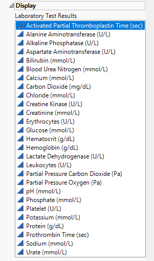
|
| Summary Statistic for Trial Data | Min | ||
| Calculate baseline using: | Last recorded pre-dose measurement | ||
| Removed unscheduled visits | unchecked | ||
| Display | Vital Signs | Diastolic Blood Pressure (mmHg) | |
| All other options set to default. | |||
This example uses the Findings Shift Plots Report to identify subjects who experienced notable decreases in diastolic blood pressure (DBP) following treatment. Such decreases may indicate a pharmacologic effect of treatment and help reviewers identify subjects who crossed clinically meaningful blood pressure thresholds.
In this example measurements taken at both scheduled as well as unscheduled visits are included. The subject’s last recorded pre-dose measurement is used as the baseline measurement. For the post-baseline measurement, the minimum recorded value for the subject was chosen. Figure 3 displays the resulting plot.
Figure 3: Basline vs. Min Post-baseline Diastolic Blood Pressure
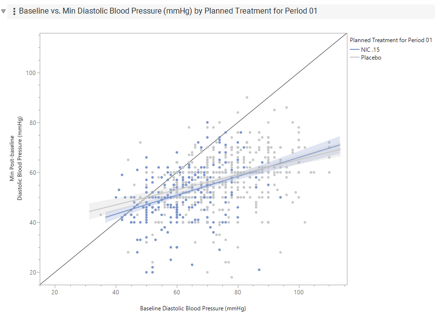
The horizontal axis displays each subject’s last pre-dose DBP measurement, while the vertical axis displays the minimum post-baseline DBP value observed during the study. The diagonal line of equality represents no change from baseline. Observations below this line indicate subjects whose minimum post-baseline DBP was lower than their baseline value. Most observations fall below the line of equality, indicating that DBP values generally decreased after treatment in both treatment groups. Several subjects experienced substantially larger decreases than the overall population, appearing as observations separated from the main cluster of points.
This plot quickly highlights subjects who experienced the greatest reductions in DBP, allowing reviewers to identify potentially clinically significant blood pressure decreases without reviewing individual listings for all subjects.
Reviewers can select regions of interest directly within the plot to identify the corresponding subjects. In this example, several subjects with large reductions in DBP were selected for further investigation (Figure 4).
Figure 4: Selecting subjects within the Basline vs. Min DBP Plot
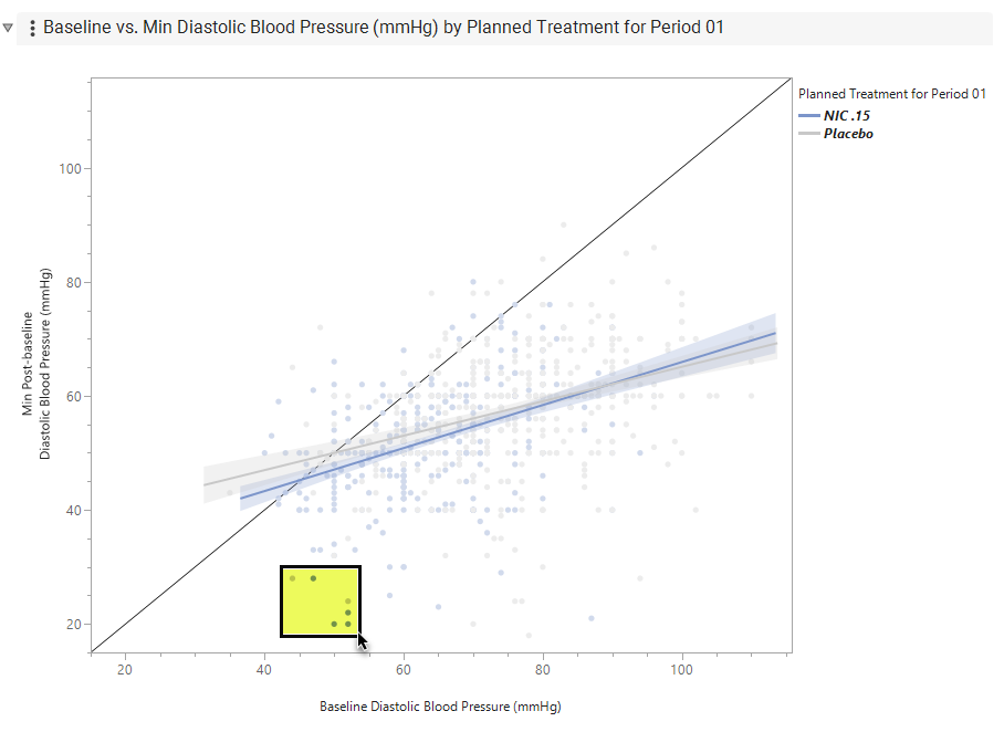
The area highlighted in yellow represents the observations selected. Click  to display the selected records in a data table (Figure 5). This table can be filtered to create a focused subject subset for detailed review (Figure 6).
Figure 5: Data table with selected subjects noted in Rows section
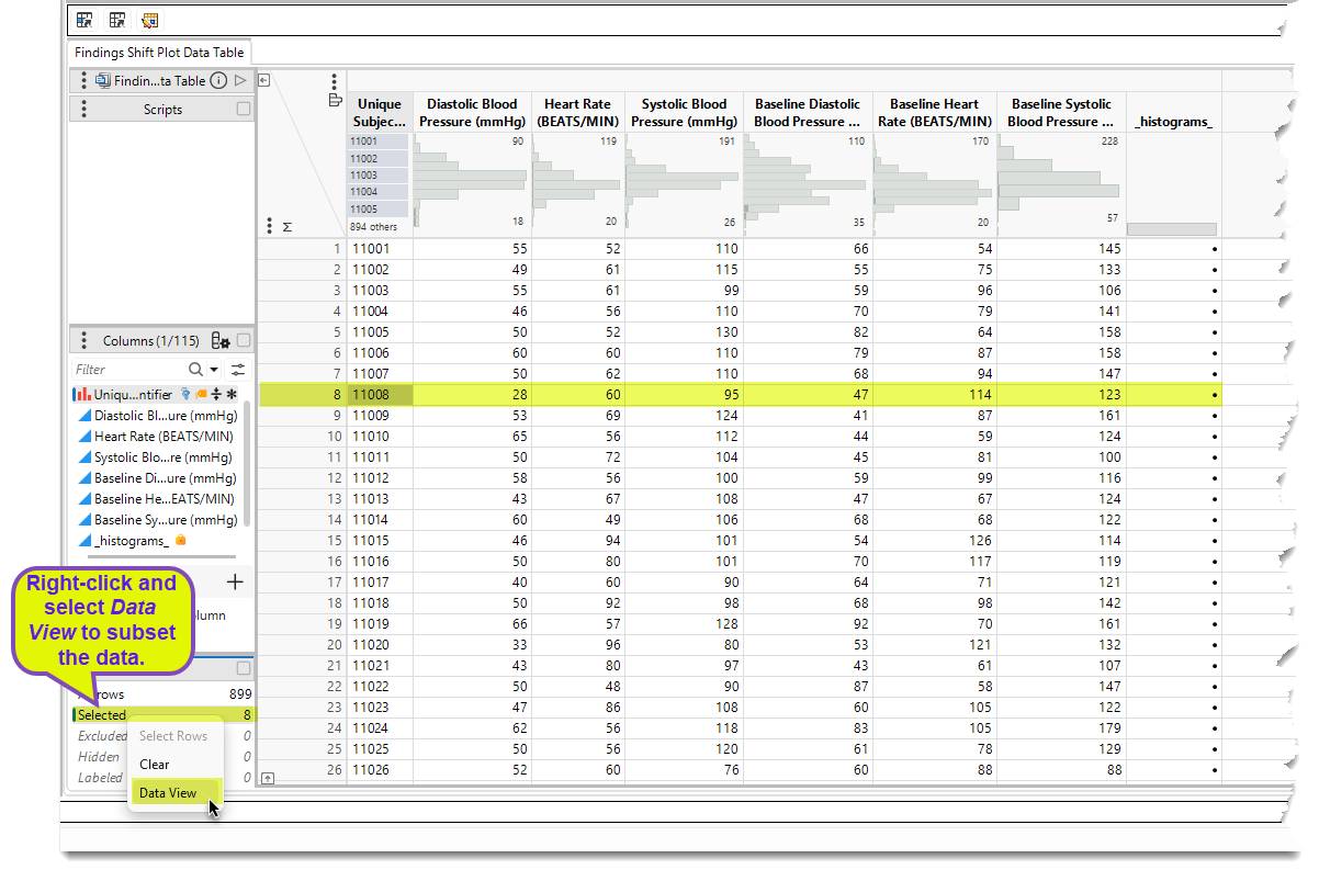
Figure 6: Subset table of selected subjects' vital signs
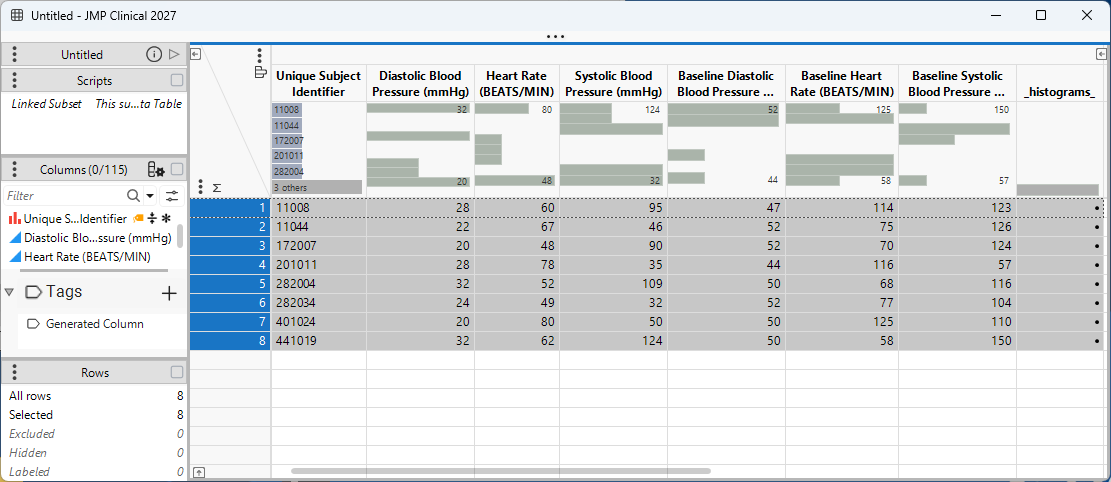
Examination of the selected subjects allows reviewers to determine whether the observed decreases are isolated findings or part of a broader pattern involving other cardiovascular measurements. Additional review of heart rate, systolic blood pressure, adverse events, and concomitant medications may help determine the clinical relevance of the observed reductions.
This example demonstrates how the Findings Shift Plots Report can rapidly identify subjects with potentially clinically meaningful decreases in blood pressure and support targeted follow-up review. By linking directly from population-level visualization to subject level data, reviewers can efficiently prioritize subjects for investigation and assess findings in the context of other vital signs and safety information. Additional review in the Patient Profiles report can provide further subject-level clinical context.
Note: You may notice a difference in baseline vital signs results between JMP Clinical v8.1 and v20. This can happen when the baseline calculation is for the mean of recorded predose measurements for findings that have "Y" as a value for VSBLF if some of those rows are missing a value for VSDY. v8.1 computes the mean for all rows that have a value of "Y" as a value for VSBLF, regardless of the value of VSDY. v20 ignores any rows lacking a value for VSDy and computes baseline means using just the rows that both have a value of "Y" as a value for VSBLF, and some value for VSDY.
Options
Data
Treatment or Comparison Variable
View/Hide Details.
Specifies the variable used to define the groups to be comparec in the report. This variableis typically a planned or actual treatment variable, such as ARM, ACTARM, TRTxxA, or TRTxxP, but it can also be another variable that defines meaningful comparison groups, such as SEX or RACE.
Select None to display the data without grouping by a treatment or comparison variable.
Domain
View/Hide Details.
Use this widget to specify whether to analyze measurements from either the Electrocardiogram (EG), Laboratory (LB), or Vital Signs (VS) findings domains.
LB is selected by default.
Findings Tests
View/Hide Details.
Use this widget to select specific Findings tests. If you leave this field blank, all tests are run.
| 8 | Click  to open the Add window (shown below) that lists available test names (shown below). to open the Add window (shown below) that lists available test names (shown below). |
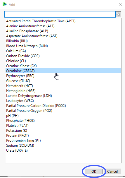
| 8 | Select the desired test(s) and click to add them to the text box. |
By Variables
View/Hide Details.
Use this field to specify one or more By variables from ADSL to use in your analysis.

Selecting a By variable will split the bar chart and tabulate by the grouping variables selected in this option as well as by the variable selected for the comparison or treatment variable.
By Variables
By variables are optional (in most reports)variable specifications whose values define groups of observations, such as hour, month, or year. BY variables can enable analyses to be performed separately on different groups as defined by that variable. Choosing a BY variable such as gender (ADSL variable = SEX), for example, groups the subjects by gender and conducts two separate analyses: one for males and one for females.
Alternatively, specifying a BY variable enables you to animate an image so that you can see how response values change according to some grouping, like over time.
To Specify One or More By Variables:
| 8 | Click to open the Add window (shown below) that lists each variable contained in domain and SUPPxx (if merged) specific to this report |
Note: In Demographics Distribution only, variables are taken from ADSL, in addition to the report-specific DS and SUPPPDS (if available) data sets.
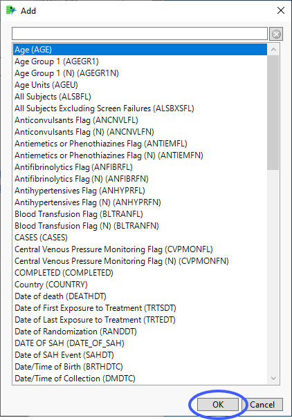
| 8 | Select the variables you want to include in the analysis and click to add those variables to the text box. |
In this example, AGE Group 1, RACE, and SEX were selected and added.
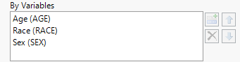
Note: If no BY variables are specified, the analysis is conducted across all the subjects
Summary Statistic for Trial Data
View/Hide Details.
Use the drop down to specify whether to display the mean (specified by default), median, maximum, minimum, or last values to summarize the results of the trial period.
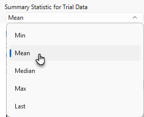
Options are defined in the following table:
|
Summary Statistic |
Definition |
||||||
|
Min |
|
||||||
|
Mean |
|
||||||
|
Median |
|
||||||
|
Max |
|
||||||
|
Last |
|
Normalization of Lab Measurements
View/Hide Details.
By default, JMP Clinical reports unaltered laboratory measurement values (None). In any cases, simply examining the raw numbers can make interpretation somewhat confusing. Normalization of Lab Measurements to accepted values can often ease these difficulties. JMP Clinical offers several methods for normalizing your data.
Note: This option is not available for domains lacking upper or lower limits of normal variables.
Use the drop-down menu to select a normalization to be applied to the baseline and on-therapy measurements.
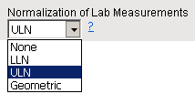
Available normalizations are described in the following table:
|
Normalization |
Definition |
|
None |
Choose this option to apply no normalization to the laboratory measurements. |
|
LLN |
Select this option to divide the measured lab values by the value considered to be the lower limit of the normal range (LLN) of values. This measure normalizes the labs relative to the LLN. Selecting this method is best used when you expect the values to fall below the normal. Normalized values less than one are considered to be lower than normal. |
|
ULN |
Select this option to divide the measured lab values by the value considered to be the upper limit of the normal range (ULN) of values. This measure normalizes the labs relative to the ULN. Selecting this option is best used when you expect the values to exceed the normal range. Normalized values greater than one are considered to be higher than normal. |
|
Geometric |
Select this option to normalize the data using the formula: normalized value = (log(x) - log(GM))/log(GSD), where x is the raw value, GM is the geometric mean of the upper limit of the normal range (ULN) of values and the lower limit of the normal range (LLN) of values, and GSD is the geometric standard deviation of the ULN and LLN. The geometric normalized data are measured on a scale (centered on 0) based on the number of GSD units the observations are from GM. On this scale the GM is the midpoint between the log transformed upper and lower limits (ULN and LLN) and each GSD is equal to half the range between the log(ULN) and log(LLN). With this normalization, values -1 and 1 are set to equal the LLN and ULN respectively and behave similar to a z-score. Clinically, values greater than 1 (or less than -1) can be interpreted as a measure of how far away the finding was from the ULN (or LLN) with respect to the normal range of values (ULN - LLN). Values less than 1 or greater than -1 would indicate that the finding was within the normal range of values. Note: This option is available only in select reports. |
log Transformation of Findings Measurements
View/Hide Details.
Log transformations can make certain response distributions closer to Gaussian with constant variance and can enable you to draw more accurate statistical conclusions under standard modeling assumptions. They are especially useful for ratio-type measurements or measurements that are always positive and skewed to the right.
Use the drop-down menu to select the transformation to be applied to the baseline and experimental measurements. None is selected by default.
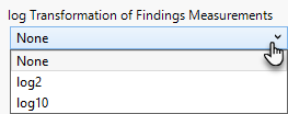
Options are listed in the following table:
|
Summary Statistic |
Definition |
|||
|
None |
|
|||
|
Log2 |
|
|||
|
Log10 |
|
Remove unscheduled visits
View/Hide Details.
You might or might not want to include unscheduled visits when you are analyzing findings by visit.
By default, this box is checked. When it is checked, records are excluded from the analysis if the VISIT variable exists and contains the text "unscheduled" for those records. If the box is not checked all records are included regardless of the VISIT status.
For some reports, you may have to specify Visits as the Time Scale to enable this field.
Calculate baseline as:
View/Hide Details.
Use this widget to use the flagged baseline record, last recorded pre-dose measurement or the mean of all the measurements taken during the baseline time window as the baseline measurement.
By default, the flagged baseline record is used.
The following test measurements are considered when forming the baseline measurement:
| • | those flagged as baseline, and |
| • | those taken prior to Study Day 1 |
Choose Last recorded pre-dose measurement to use the last recorded pre-dose test measurement (out of the test measurement pool generated from the above list) as the baseline measurement.
Choose Mean of recorded pre-dose measurements to average these pre-dose test measurements to form the baseline measurement.
Note: When the selected option to calculate baseline is to use the baseline flag and there are two records flagged as baseline, JMP Clinical uses the last record. This differs from JMP Clinical version 8.1, wherein the mean of the flagged baseline values was used.
Snapshot Records to Include
View/Hide Details.
Use this widget to specify which updated snapshot records to include in your analysis. This option is surfaced only in studies where the number of snapshots is greater than 0.
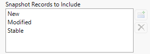
The default state of this option is to show new, modified and stable - effectively all - snapshot records. To see specific records you must remove undesired records from the analysis. For example, to surface only the new records, select both Modified and Stable and click  . Click
  to restore deleted records.
Note: JMP Clinical now relies on the JMP Compare Data Tables platform to detect new records. When duplicate rows appear, the platform evaluates them based on their row order. As a result, records are no longer labeled as Non‑Unique or Previously Non‑Unique, and the corresponding options to include those records have been removed.
Additional Filters - Findings
View/Hide Details.
This filter lets you restrict your analysis to only those subjects that meet specific criteria at the level of the specified Findings domain (EG, LB, or VS) .

This filters uses JMP WHERE clauses to Select Rows that meet the specified criteria. To use this filter, you must enter the JSL (JMP Scripting Language) expressions that constitute the WHERE clause in the appropriate text box for specific filtering of findings. Note: This is an advanced concept that not only requires some basic knowledge of the JSL where clause syntax (similar to, but different from, SQL), but also an understanding of the exact variables in the tables in the study.
Risk indicators are calculated using this subset only.
To specify a Findings filter:
| 8 | Click  to open the Where Clause Builder to construct the desired filter. to open the Where Clause Builder to construct the desired filter. |
| 8 | Click  to clear the filter. to clear the filter. |
Note: To filter subjects with a specific event or finding, one could also use the Subpopulation Builder on any domain of interest. For example, filter to all subjects that exhibit cardiac failure ( :Customized Query 01 Name == "Cardiac failure" ) and run all reports on those.
Display
Test Results/Vital Signs
View/Hide Details.
This option lists all of the tests performed over the course of the study. The list is specific to the selected Findings domain and changes when you change the selected domain.
| 8 | Select one or more tests to display only the results for the selected domain(s). |
Action Buttons
Action buttons provide you with an easy way to drill down into your data. The following action buttons are generated by this report:
Click here to display the list and description of the Report Action buttons.
| • | Click  to rerun the report using default settings. to rerun the report using default settings. |
| • | Click  to view the associated data tables. Refer to Show Tables for more information. to view the associated data tables. Refer to Show Tables for more information. |
| • | Click  to generate a standardized PDF- or RTF-formatted report containing the plots and charts of selected sections. to generate a standardized PDF- or RTF-formatted report containing the plots and charts of selected sections. |
| • | Click  to generate a JMP Live report. Refer to Create Live Report for more information. to generate a JMP Live report. Refer to Create Live Report for more information. |
| • | Click  to take notes, and store them in a central location. Refer to Add Notes for more information. to take notes, and store them in a central location. Refer to Add Notes for more information. |
| • | Click  to read user-generated notes. Refer to View Notes for more information. to read user-generated notes. Refer to View Notes for more information. |
| • | Select one or more subjects, then click  to apply the Review Subject Filter and filter all reports in the review builder on the selected subjects. to apply the Review Subject Filter and filter all reports in the review builder on the selected subjects. |
| • | Select a group of subjects and click  to specify Derived Population Flags that enable you to distinguish the selected group of subjects from the general population. to specify Derived Population Flags that enable you to distinguish the selected group of subjects from the general population. |
Default Settings
Refer to Set Study Preferences for default Subject Level settings.