Results
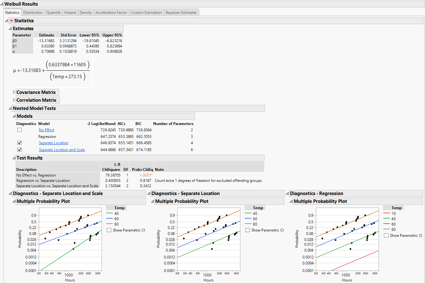
The Results section of the report window shows more detailed statistics and prediction profilers than those shown in the Comparisons report. Separate result sections are shown for each selected distribution. Figure 4.13 shows a portion of the Weibull results, Nested Model Tests, and Diagnostics plots for Devalt.jmp.
Statistical results, diagnostic plots, and Distribution, Quantile, Hazard, Density, and Acceleration Factor Profilers are included for each of your specified distributions. The Custom Estimation tab lets you estimate specific failure probabilities and quantiles, using both Wald and Profile interval methods. When the Box-Cox Relationship is selected on the platform launch window, the Sensitivity tab appears. This tab shows how the Relative Log-likelihood and B10 Life change as a function of Box-Cox lambda.
Figure 4.13 Weibull Distribution Nested Model Tests for Devalt.jmp Data
Statistics
For each parametric distribution, there is a Statistics section that shows parameter estimates, a covariance matrix, confidence intervals, summary statistics, and diagnostic plots. You can save probability, quantile, and hazard estimates by selecting any or all of these options from the Statistics red triangle menu for each parametric distribution. The estimates and the corresponding lower and upper confidence limits are saved as columns in your data table. Figure 4.14 shows the save options available for any parametric distribution.
Figure 4.14 Save Options for Parametric Distribution
Nested Model Tests
Nested Model Tests are included, if you selected the option on the platform launch window. The Nested Model Tests include statistics and diagnostic plots for the following models:
Separate Location and Scale
Assumes that the location and scale parameters are different for all levels of the explanatory variable. This option is equivalent to fitting the distribution by the levels of the explanatory variable. The Separate Location and Scale model has multiple location parameters and multiple scale parameters (Figure 4.15).
Separate Location
Assumes that the location parameters are different, but the scale parameters are the same for all levels of the explanatory variable. The Separate Location model has multiple location parameters and only one scale parameter (Figure 4.16).
Regression
The default model shown in the initial Fit Life by X report window (Figure 4.17).
No Effect
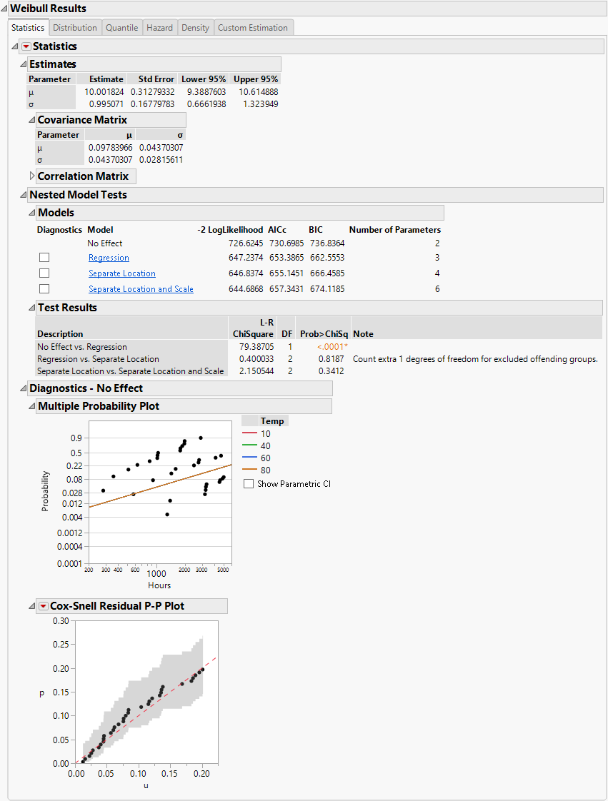
Assumes that the explanatory variable does not affect the response. This option is equivalent to fitting all of the data values to the selected distribution. The No Effect Model has one location parameter and one scale parameter (Figure 4.18).
Separate Location and Scale, Separate Location, and Regression analyses results are shown by default. Regression parameter estimates and the location parameter formula are shown under the Estimates section, by default. The Diagnostics plots for the No Effect model can be displayed by selecting the check box to the left of No Effect under the Nested Model Tests title.
To see results for each of the models (independently of the other models), click the underlined model of interest (listed under Nested Model Tests) and then uncheck the check boxes for the other models.
If the Nested Model Tests option was not checked in the launch window, then the Separate Location and Scale and Separate Location models are not assessed. In this case, estimates are given for the regression model for each distribution that you select and the Cox-Snell Residual P-P Plot is the only diagnostic plot.
Note: When Separate Location and Scale or Separate Location models are fit for the Weibull distribution, both parameterizations of the Weibull distribution are shown in the Estimates table, as is the case in Figure 4.15 and Figure 4.16. For more information about the Weibull parameterizations, see Weibull in the Survival Analysis section.
Diagnostics
The Multiple Probability Plots shown in Figure 4.13 are used to validate the distributional assumption for the different levels of the accelerating variable. If the line for each level does not run through the data points for that level, the distributional assumption might not hold. Side-by-side comparisons of the diagnostic plots provide a visual comparison for the validity of the different models. See Meeker and Escobar (1998, sec. 19.2.2) for a discussion of multiple probability plots. Each multiple probability plot has an option below the legend that enables you to show or hide shaded parametric confidence intervals for each line in the plot.
The Cox-Snell Residual P-P Plots are used to validate the distributional assumption for the data. If the data points deviate far from the diagonal, then the distributional assumption might be violated. The Cox-Snell Residual P-P Plot red triangle menu has an option called Save Residuals that enables you to save the residual data to the data table. See Meeker and Escobar (1998, sec. 17.6.1) for a discussion of Cox-Snell residuals.
Figure 4.15 Separate Location and Scale Model with the Weibull Distribution for Devalt.jmp Data
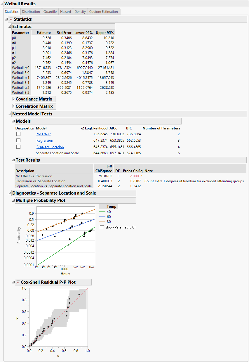
Figure 4.16 Separate Location Model with the Weibull Distribution for Devalt.jmp Data
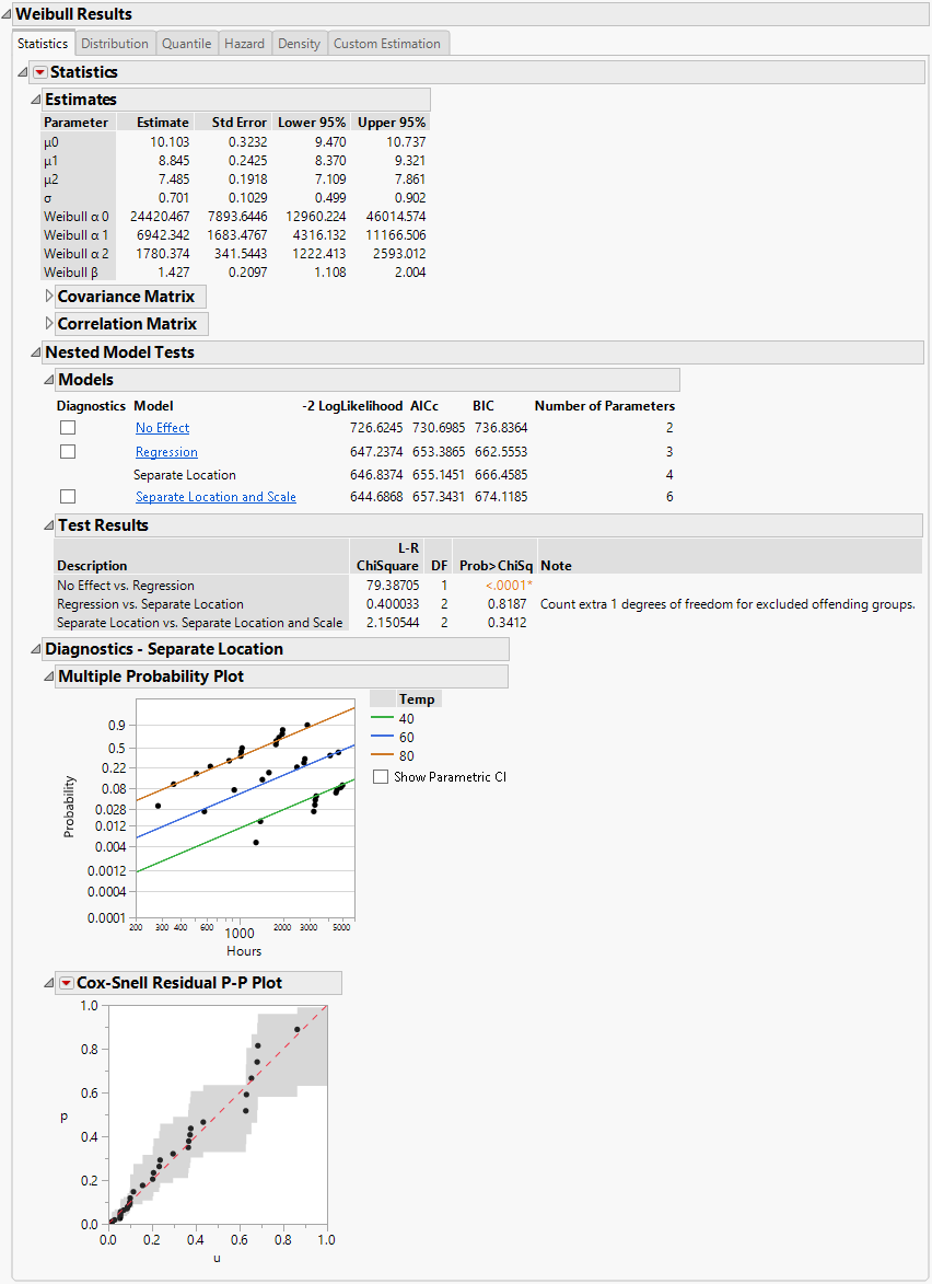
Figure 4.17 Regression Model with the Weibull Distribution for Devalt.jmp Data
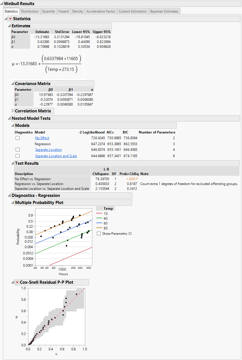
Figure 4.18 No Effect Model with the Weibull Distribution for Devalt.jmp Data
Profilers and Surface Plots
In addition to a statistical summary and diagnostic plots, the Fit Life by X report window also includes profilers and surface plots for each of your specified distributions. To view the Weibull time-accelerating factor and explanatory variable profilers, click the Distribution tab under Weibull Results. To see the surface plot, click the disclosure icon to the left of the Weibull title (under the profilers). The profilers and surface plot behave similarly to other platforms. See Profiler and Surface Plot in Profilers.
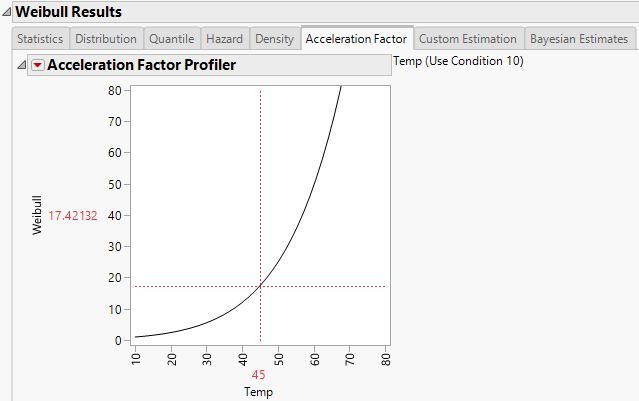
The report window also includes a tab labeled Acceleration Factor. Clicking the Acceleration Factor tab shows the Acceleration Factor Profiler. This profiler is an enlargement of the Weibull plot shown under the Acceleration Factor tab in the Comparisons section of the report window. Figure 4.19 shows the Acceleration Factor Profiler for the Weibull distribution of Devalt.jmp. The use condition level for the explanatory variable can be modified by selecting the Set Time Acceleration Use Condition option in the Fit Life by X red triangle menu.
Figure 4.19 Weibull Acceleration Factor Profiler for Devalt.jmp
Custom Estimation
For each parametric distribution, there is a Custom Estimation section that contains two reports: Estimate Quantile and Estimate Probability. The Estimate Quantile report contains a calculator that enables you to predict quantiles for specific failure probability values. The Estimate Probability report contains a calculator that enables you to predict failure and survival probabilities for specific time values. Both Wald-based and likelihood-based confidence intervals are available for each estimated quantity. The confidence level for these intervals is determined by the Change Confidence Level option in the Fit Life by X red triangle menu.
Estimate Quantile
In the Estimate Quantile calculator, enter a value for Prob and the X variable. Press Enter to see the quantile estimates and corresponding confidence intervals. To calculate multiple quantile estimates, click the plus sign, enter another Prob value, another X value, or both, and press Enter. Click the minus sign to remove the last entry. If you enter more than one value in either column, the table contains all combinations of Prob and X values.
By default, Wald-based intervals are shown. Click Likelihood CI in the Interval Type outline to switch to likelihood-based confidence intervals.
Estimate Probability
In the Estimate Probability calculator, enter a value for Time and the X variable. Press Enter to see the failure probability estimates and corresponding confidence intervals. To calculate multiple failure probability estimates, click the plus sign, enter another Time value, another X value, or both, and press Enter. Click the minus sign to remove the last entry. If you enter more than one value in either column, the table contains all combinations of Time and X values.
By default, Wald-based intervals are shown. Click Likelihood CI in the Interval Type outline to switch to likelihood-based confidence intervals.
Bayesian Estimates
For each parametric distribution other than Exponential, there is a Bayesian Estimates section that enables you to obtain Bayesian parameter estimates. The Bayesian Estimates section is not available if the Relationship in the Fit Life by X launch window is Custom, No Effect, Location, or Location and Scale.
Bayesian estimation in the Fit Life by X platform is done using a Markov Chain Monte Carlo (MCMC) algorithm. More specifically, the platform attempts a basic rejection sampler. If the rejection sampler produces valid results, these results are reported. If the rejection sampler cannot produce valid results, the platform uses a random walk Metropolis-Hastings algorithm and adds a note to the top of the Bayesian Estimation report. See Robert and Casella (2004).
The initial report is a control panel where you can specify prior distributions for the parameters and control aspects of the simulation. To obtain posterior estimates of the parameters, specify the prior distributions and the simulation options, and then click Fit Model.
To specify the prior distributions of the parameters, you must specify information about a quantile of the distribution and the slope β1 and scale σ parameters. (For the Weibull distribution, you specify the Weibull β rather than σ.) The quantile is defined by two values: the probability of the quantile and the value of the X variable at the specified quantile. The default Probability value is 0.10, but you can specify a value that corresponds to the quantile of interest. Specify information about the range of the prior distribution. For Normal and Lognormal prior distributions, the range is specified in terms of Lower and Upper 99% limits. For Uniform and Log-Uniform prior distributions, the range is specified in terms of the Lower and Upper limits. See Meeker and Escobar (1998). The initial values that are provided are estimates consistent with the maximum likelihood estimates in the Statistics section of the report.
The following options for the simulation appear below the prior distribution specification table:
Number of Monte Carlo Iterations
Sets the sample size that will be drawn from the posterior distribution after a burn-in procedure is completed.
Random Seed
Sets the initial state of the simulation. By default, it is the clock time. The number should be a positive integer greater than 1. If you specify 1, the current clock time is used.
Bayesian Estimates - Result <N> Report
After you specify prior distributions and the simulation options, click Fit Model to perform the simulation. A Bayesian Estimates - Result <N> report is provided for each simulation. This report contains the following headings:
Priors
Shows the specifications that you entered in the Bayesian Estimates report to run the simulation. The Prior report also contains the random seed.
Posterior Estimates
Shows five marginal statistics and one joint statistic describing the posterior distribution of β0, β1, σ, and the quantile. The marginal statistics are the median, 0.025 quantile (Lower Bound), 0.975 quantile (Upper Bound), mean, and standard deviation computed from the Monte Carlo samples. The parameter values listed beneath Joint HPD are the values where the joint posterior density is maximized. If the Weibull distribution is specified, this table contains the posterior estimate of the Weibull β instead of σ.
To compute statistics for other derived variables based on the posterior estimates of the generic parameters, click the Export Monte Carlo Samples link.
Posterior Scatter Plot
Shows two scatter plots of values from the Monte Carlo simulation. The scatter plot on the left shows the values of the posterior parameters as they are specified in the Priors report. The scatter plot on the right shows the values of the posterior parameters as they are specified in the Posterior Estimates report.
Profilers
Shows two profilers based on samples from the posterior distribution. The values shown in the profilers, at the specified values of the X and Time variables, are calculated as follows:
– For each set of sampled parameter values from the posterior distribution, the values of the cumulative distribution function and the quantile function are calculated at the specified values of the X and Time variables.
– The predicted values of the cumulative distribution function and the quantile function are the medians of the calculated values.
– The upper and lower confidence limits are the 0.025 and 0.975 quantiles of the calculated values. The confidence level for these limits is determined by the Change Confidence Level option in the Fit Life by X red triangle menu.
Distribution Profiler
Shows the parametric cumulative distribution function as a function of the X variable and Time.
Quantile Profiler
Shows the parametric quantile function as a function of the X variable and a specified probability.
Bayesian Estimates - Result <N> Options
The Bayesian Estimates - Result <N> red triangle menu contains the following options:
Remove
Removes the current Bayesian Estimates report from the Fit Life by X report.
Export Monte Carlo Samples
Saves the results of the Monte Carlo simulation to a new data table. You can use this table to compute statistics of the posterior estimates.