Create Cross Domain Data
This report creates indicator variables from various domains and appends to the ADSL table to create a new cross domain data table. Options exist to create indicator variables from interventions domains (e.g. CM, SU), events domains (e.g AE, MH, CE), binary variables in ADSL, character findings (e.g. VSSTRESC in VS domain) and high and low laboratory tests (LBTESTCD in LB domain). Summary statistic variables (Max, Min, Mean, Median, Last) for numeric findings (XXSTRESN in XX findings domain) will also be created when corresponding options are checked. The report converts all character variables with values N and Y to numeric variables with values 0 and 1, respectively. The resulting output data set is suitable for pattern discovery and predictive modeling. A transposed version of the data set is also produced. Both versions are useful for clustering.
Report Results Description
Running this report with the Nicardipine sample setting generates the Results shown below. Output from the report is organized into sections. Each section contains one or more plots, data panels, data filters, or other elements that facilitate your analysis.
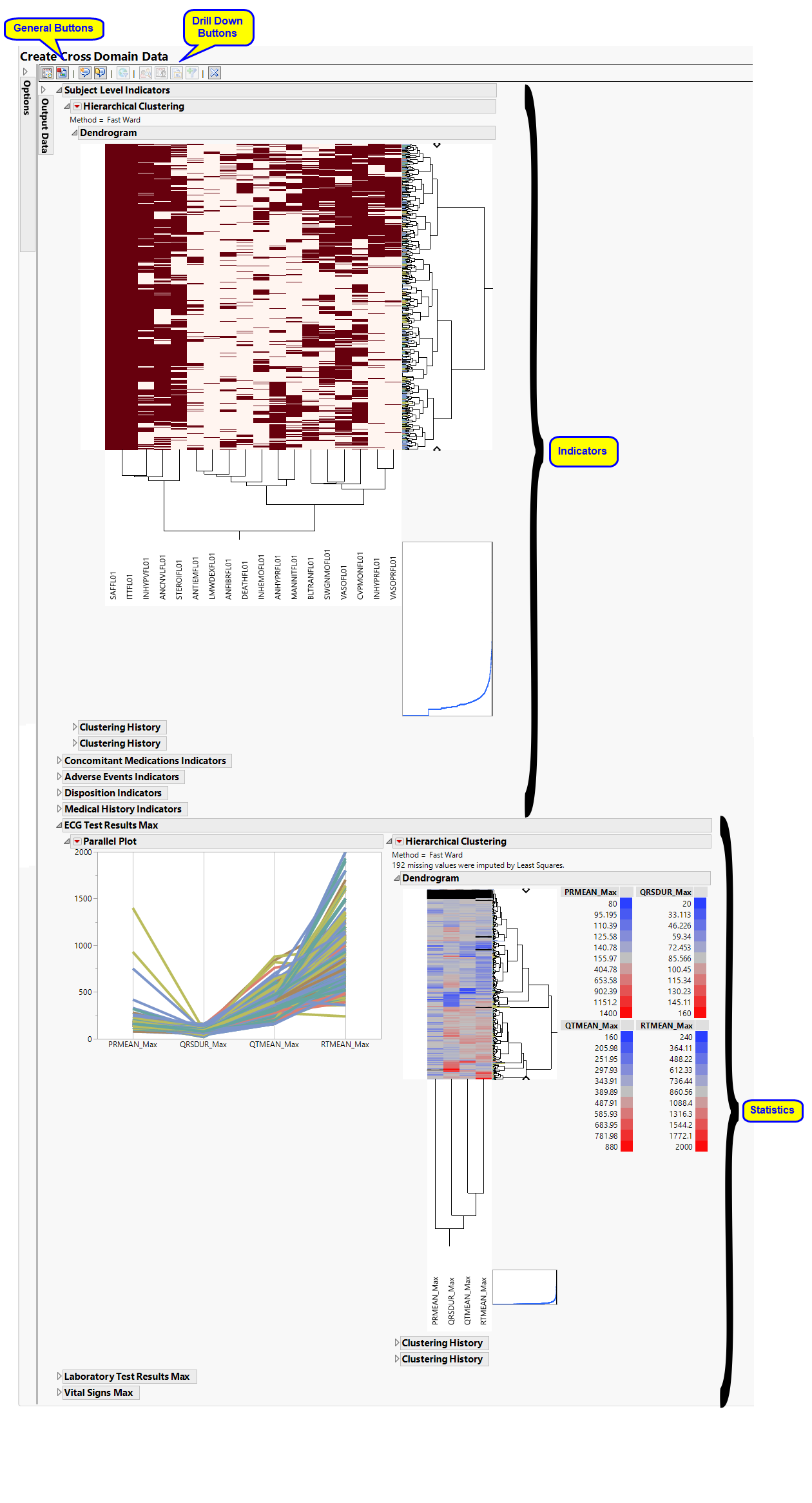
The Create Cross Domain Data report initially shows two sections Indicators and Statistics. Use the available options in each section to drill-down into the data.
Indicators
Hierarchically clusters all binary indicator variables. A separate section is created for each domain (ADSL(Subject Level), Concomitant Medications (CM), Adverse Events (AE), Disposition (DS), and Medical History (MH)) that has binary variables, depending on the options selected. The binary variables are converted to 0s and 1s and clustered.
The AD Indicators section is shown below:
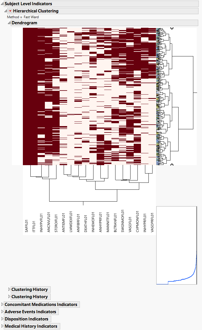
An Indicator section contains the following elements:
| • | A two-way hierarchical clustering analysis of the 0-1 variables, with subjects as rows and indicator variables as columns. |
You can study the Heat Map and Dendrogram to see both subjects that have similar values of the binary variables as well as binary variables that are similar across subjects.
See the JMP Hierarchical Clustering platform for more information.
Statistics
Hierarchically clusters a statistic computed on continuous variables. A separate section is created for each domain (ECG Test Results (EG), Laboratory Test Results (LB), and Vital Signs (VS)) that has continuous variables.
The EG Max section is shown below:
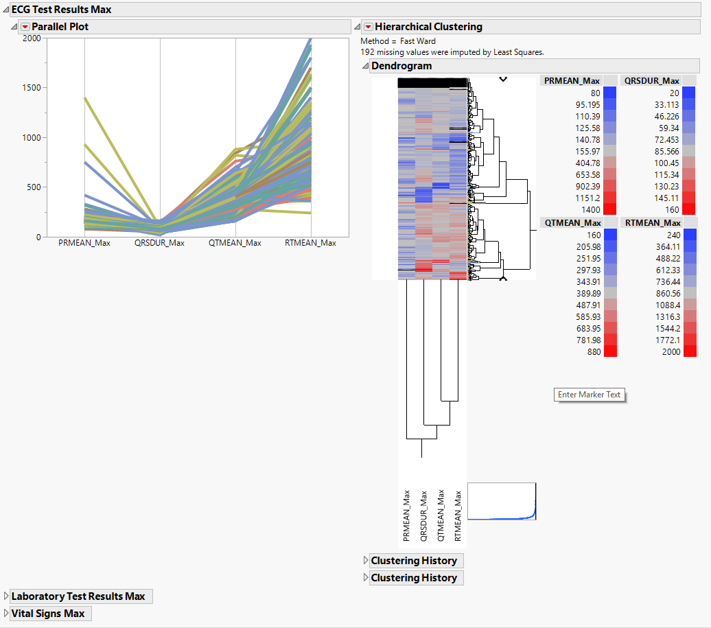
Statistics sections contains the following elements:
| • | Parallel Plot |
This shows a Parallel Plot of the computed statistic for each variable in the domain. Each line in the plot corresponds to a subject. In the example above, the max statistic is plotted for four variables. The coloring of the lines comes from the hierarchical clustering analysis of the first numeric domain.
You can study this plot to determine trends across variables as well as outlying subjects.
See the JMP Parallel Plot platform for more information.
| • | Hierarchical Clustering |
This displays a two-way clustering analysis of the statistic across all variables and subjects.
You can study this plot to determine numeric measurements that are similar across subjects and/or subjects that are similar across numeric measurements.
See the JMP Hierarchical Clustering platform for more information.
Output Data
This pane provides links to the following output data sets:
| • | Transposed Subject Data (adsl_cddt.sas7bdat): This data set is the transpose of the main output table. The transposed table has domain data identifiers as rows and subjects as columns. |
Action Buttons
Action buttons, provide you with an easy way to drill down into your data. The following action buttons are generated by this report:
| • | Profile Subjects: Select subjects and click  to generate the patient profiles. See Profile Subjects for additional information. to generate the patient profiles. See Profile Subjects for additional information. |
| • | Show Subjects: Select subjects and click  to open the ADSL (or DM if ADSL is unavailable) of selected subjects. to open the ADSL (or DM if ADSL is unavailable) of selected subjects. |
| • | Adverse Events Narrative Generation: Select subjects and click  to open the Adverse Events Narrative dialog. From this dialog, you can customize options and generate a narrative. to open the Adverse Events Narrative dialog. From this dialog, you can customize options and generate a narrative. |
| • | Create Subject Filter: Select subjects and click  to create a data set of USUBJIDs for subjects experiencing selected events, which subsets all subsequently run reports to those selected subjects. The currently available filter data set can be applied by selecting Apply Subject Filter in any report dialog. to create a data set of USUBJIDs for subjects experiencing selected events, which subsets all subsequently run reports to those selected subjects. The currently available filter data set can be applied by selecting Apply Subject Filter in any report dialog. |
General
| • | Click  to view the associated data tables. Refer to View Data for more information. to view the associated data tables. Refer to View Data for more information. |
| • | Click  to generate a standardized pdf- or rtf-formatted report containing the plots and charts of selected sections. to generate a standardized pdf- or rtf-formatted report containing the plots and charts of selected sections. |
| • | Click  to generate a JMP Live report. Refer to Create Live Report for more information. to generate a JMP Live report. Refer to Create Live Report for more information. |
| • | Click  to take notes, and store them in a central location. Refer to Add Notes for more information. to take notes, and store them in a central location. Refer to Add Notes for more information. |
| • | Click  to read user-generated notes. Refer to View Notes for more information. to read user-generated notes. Refer to View Notes for more information. |
| • | Click  to open and view the Subject Explorer/Review Subject Filter. to open and view the Subject Explorer/Review Subject Filter. |
| • | Click  to specify Derived Population Flags that enable you to divided the subject population into two distinct groups based on whether they meet very specific criteria. to specify Derived Population Flags that enable you to divided the subject population into two distinct groups based on whether they meet very specific criteria. |
| • | Click the arrow to reopen the completed report dialog used to generate this output. |
| • | Click the gray border to the left of the Options tab to open a dynamic report navigator that lists all of the reports in the review. Refer to Report Navigator for more information. |
Report Options
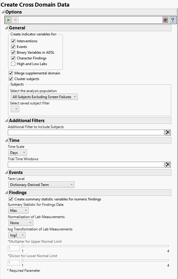
Indicator Variables
Indicator variables are binary variables whose values 1 and 0 respectively indicate a Yes or No response.
Use the indicator variable options to generate additional variables that indicate whether specific Interventions have been made, specific Events have occurred, and/or High and Low Labs results have been observed. In addition, indicator variables can be created for Binary Variables in ADSL as well as Character Findings in SDTM.
Note: If you choose to create indicator variables for High and Low Labs, you must also specify the Multiplier for Upper Normal Limit and the Divisor for Lower Normal Limit below.
Supplemental Data
This report currently allows you to make a term level selection for events that sometimes includes variables that are in a supplemental domain (SUPPXX) associated with your study. In this case, you can use the Merge supplemental domain option to merge the non-standard data contained therein into your data.
Clustering
Use the Cluster subjects option to perform subject-level clustering for each domain.
Filtering the Data:
Filters enable you to restrict the analysis to a specific subset of subjects based on values within variables. You can also filter based on population flags (Safety is selected by default) within the study data.
See Select the analysis population, Select saved subject filter1, Additional Filter to Include Subjects, and Subset of Visits to Analyze for Findings for more information.
Time Windows
By default, time is measured by visits. However, you can change the Time Scale to measure time in either weeks or days. This option is useful for assessing report graphics for exceptionally long studies.
When analyzing findings results by either days or weeks instead of by visit, you must specify the start and end days for each of one or more time windows. Trial Time Windows are defined blocks of time within the study where findings results are considered in a single time point regardless of where within the window, they were collected.
Events
The term levels are determined by the coding dictionary for the Event domain of interest; typically these levels follow the MedDRA dictionary. You must indicate how each adverse event is named . For example, selecting Reported Term as the Term Level reports the event specified by the actual event term as reported in the AE domain.
Findings
Summary Statistics
Select the Create summary statistic variables for numeric findings to generate a new column containing the specified Summary Statistic for Findings Data for the numeric findings in each of the selected findings domains. Available summary statistics include Mean, Median, Maximum, Minimum, and Last Recorded Value.
Normalization
By default, JMP Clinical reports unaltered laboratory measurement values. In any cases, simply examining the raw numbers can make interpretation somewhat confusing. Normalization of Lab Measurements to accepted values can often ease these difficulties. JMP Clinical offers three options for normalizing your data.
Selecting LLN normalizes the data to the lower limit of the expected normal range and is best used when you expect the values to fall below the normal. Normalized values less than one are considered to be lower than normal.
Selecting ULN normalizes the data to the upper limit of the expected normal range and is best used when you expect the values to exceed the normal range. Normalized values greater than one are considered to be higher than normal.
Selecting Geometric normalizes the data such that the lower limit of the expected normal range is set to -1 and the upper limit of the expected normal range is set to +1. This method is best used when there is no expectations of where the values might fall. Normalized values less than -1 are considered to be lower than normal while values greater that +1 are higher than normal.
Log transformations can make certain response distributions closer to Gaussian with constant variance and can enable you to draw more accurate statistical conclusions under standard modeling assumptions. They are especially useful for ratio-type measurements or measurements that are always positive and skewed to the right. You can use the log Transformation of Lab Measurements options to either use non-transformed data or to log2- or log10-transform your measurements.
High and Low Labs
Use the Multiplier for Upper Normal Limit and Divisor for Lower Normal Limit options to define the range above and below which findings results are considered abnormally high or low, respectively.